Thousands of animals are present in shelter homes and much more are present on the
streets. In order to stop things like cruelty and euthanization of these animals, we
need to increase animal adoption rates. Animals with cute pictures are more likely to
get adopted. Shelters need a way to estimate and increase “cuteness” of
photos of these animals to get them adobted faster. The goal of our project is to use
machine learning to make accurate predictions of “cuteness” and increase animal adoption
rates from the shelters.
Problem definition
For CS7641, our project aims at estimating the cuteness/popularity of images of shelter animals.
This is an open kaggle
challenge.
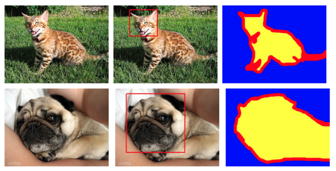
The dataset contains raw images of shelter animals along with metadata.
The metadata consists of a set of binary features like presence of eyes, face, etc.
In this project, we use both supervised learning and unsupervised learning to estimate
popularity/cuteness of images. In particular, we use representation learning to learn features
from raw images along with PCA to select prominent features from the metadata. Finally, we plan
on demonstrating the effectiveness of our solution by plotting training and validation loss
along with an ablation study.
Dataset exploration and visusalizations
The dataset consists of:
Images:
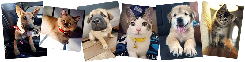
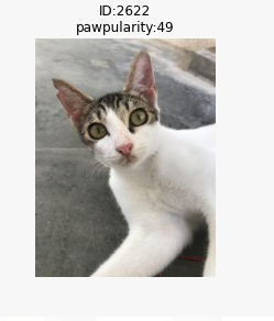
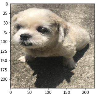
A training data set of close to \(10,000\) RGB images. Each image has a pawpularity score
as shown in [Fig 1] [Fig 1] Example image data available in the dataset
Each image has a score [the pawpularity score] which represents the perceived cuteness of a pet from the image.
This score lies in the range of 0-100. The image below shows the distribution of the score in the entire dataset.
[Fig 2] Distribution of pawpularity scores
Metadata:
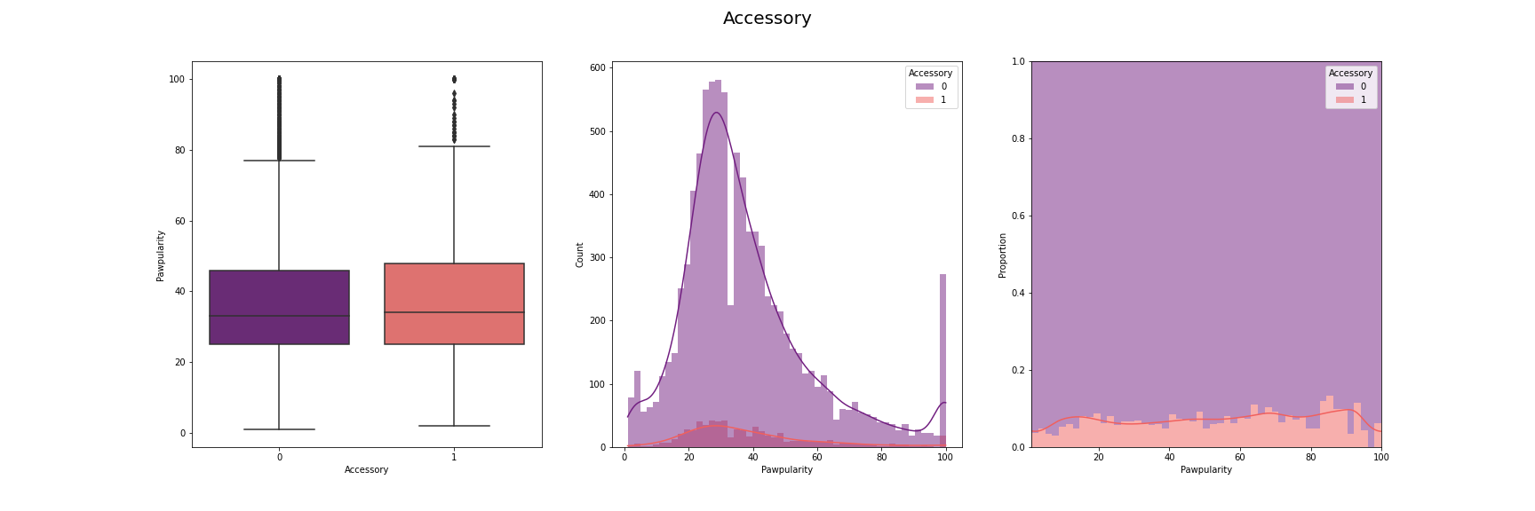
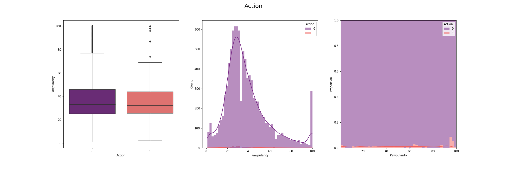
For each image in the training set, we also have a set of metadata available. The
information regarding the following twelve binary features: Focus, Eyes, Face, Near,
Action, Accessory, Group, Collage, Human, Occlusion, Info, Blur.
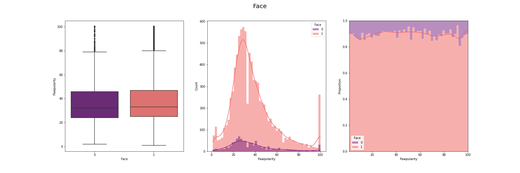
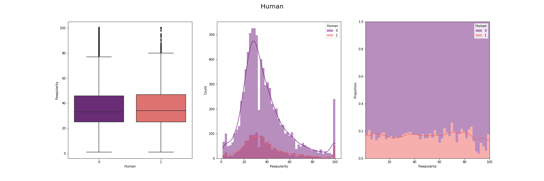
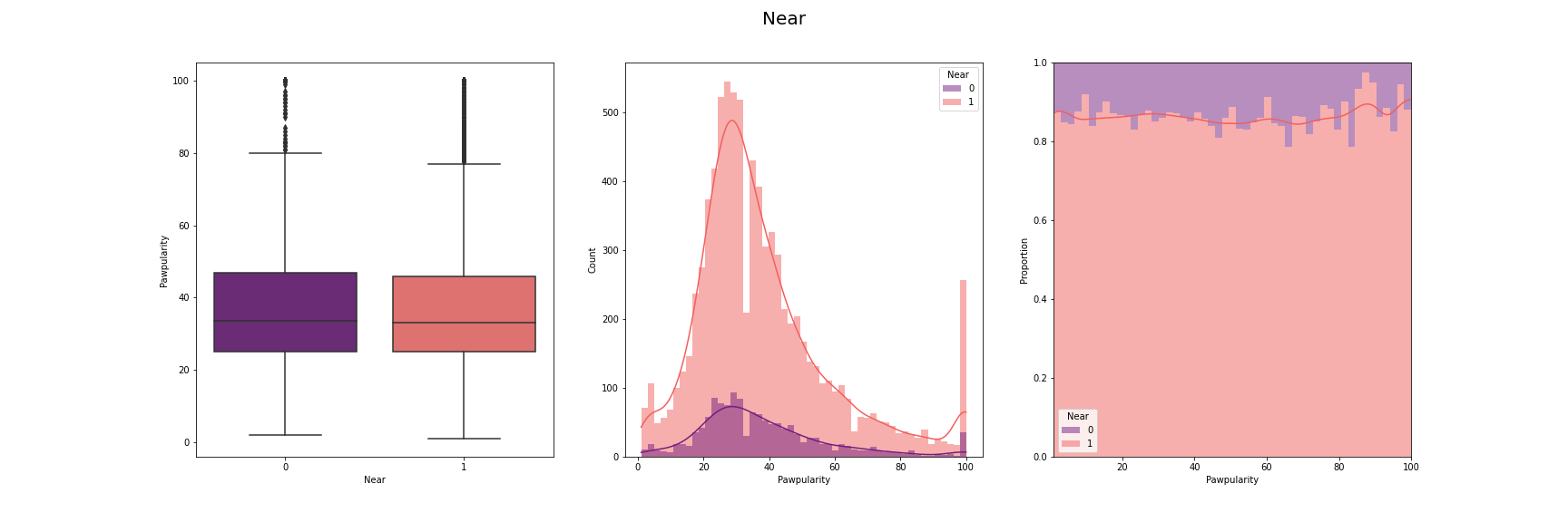
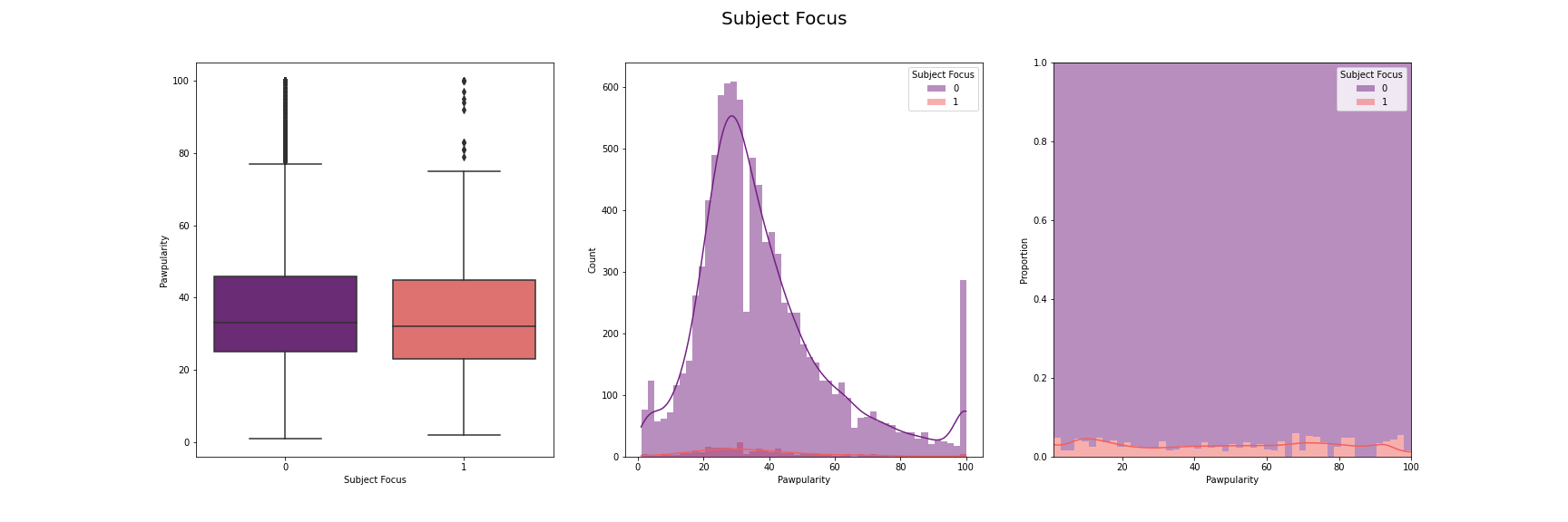
We have visualised the distribution of pawpularity with respect to each of the features.
For this, we have used box-plot, histogram and proportion of presence and absence of
each feature for each pawpularity levels. We have used modifications of the method
described in [7] for the visusalizations. The distributions for each of the features are
given below:
[Fig 3] The distribution of pawpularity score w.r.t. each of the features
As we can see from the charts, the the distributions of the pawpularity scores does not vary
much across the positive and negative states of the features. The proportions of the positive
and negative states of the features remain almost constant throughtout all values of
pawpularity. This is consistent with our analysis in other stages shared in [Fig 3] where we
found almost no correlation within the metadata and pawpularity.
Models using metadata for training
Linear Regression:
The metadata was split into a 80-20 share for the purposes of training and validation.
All results reported are for the validation set.
Without PCA:
We first ran Linear Regression on the metadata. However, the \(R^2\) score of the
regressor turned out to be very poor at only \(0.003\). This meant that the
variation in the input features did not explain the variation in target.
Additionally, the RMSE score was \(20.4944\).
With PCA [Unsupervised Learning]:
We next ran PCA on the meta-data with an intention to retain \(90\)% of the variance
in data. We then again ran the transformed features against the target variables.
This reduced the \(R^2\) of the model to an even lower value of \(0.0001\).
We also used lightgbm on the metadata to verify if introduction of non-linearilty
improves the regression scores.
However, the rmse score stayed at \(~20\). The best RMSE score we were able to achieve
using lightgbm was \(20.466760\)
The outputs of the Linear Regressor as well as the results of our initial data visualization
[Fig 2]
worsened our confidence on the viability of using metadata for training. Therefore, we
checked the correlation of the input features with the target data. The results indicated
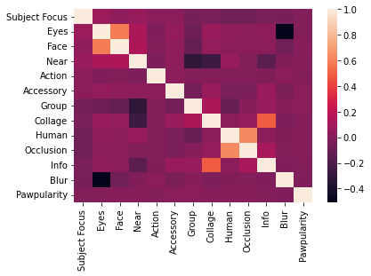
that the metadata contained practically zero correlation with the metadata as can be seen in
the [Fig 3] and there is not much information value in the metadata. [Fig 4] Correlation Matrix
With this we shifted our focus to train the model with the image data only.
Models using images for training
Attempt 1: Tuned Resnet18
Our initial attempt was to create the regressor by creating a modification of the Resnet18 model.
The preprocessing step consisted of:
Converting all the RBG images \((0,255)\) to pytorch tenors with values scaled to \((0,1)\)
Resizeing all images to \(256\times256\) pixels as images had different sizes by averaging
nearby pixels to get the required size.
We also normalized all the images with a mean of \((0.485, 0.456, 0.406)\) and std of \((0.229,
0.224, 0.225)\) which are determined to give better performance on imagenet models like resnet18
etc based on the imagenet image statistics
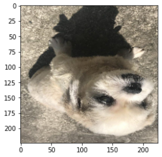
Unsupervised method to remove duplicates:
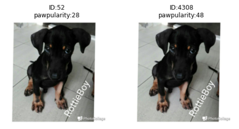
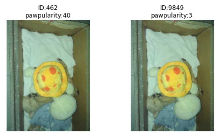
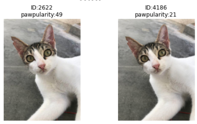
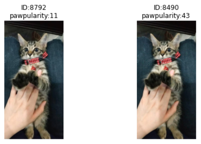
While manually inspecting the image data we also found that the dataset has a lot of noise.
Individually looking at the photos, we noticed that the popularity score did not always
tally with the cuteness/quality of the animal. In addition to this, we also noticed that
there are several duplicate images with different popularity scores in the dataset.
Given this new found knowledge, we tried multiple ways to mitigate this. The final
solution was to write a small script to extract the duplicate images by cosine
similarity between the pairs of images. We chose to flatten the image and then found the
similarity between two images using the formula: \(a.b / |a||b|\)
The images below show a sample of the duplicate images with contradictory pawpularity
scores that we were able to find.
[Fig 5] Some examples of duplicate images To help with training, we chose to exclude these images from our training and test set.
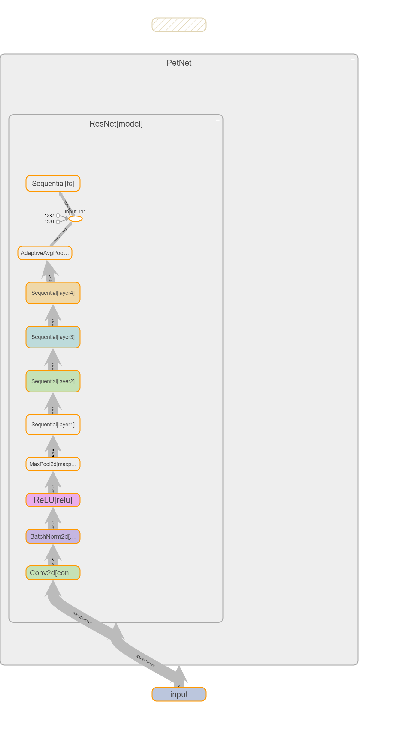
The final model architecture of the DNN to perform regression on the image data is as below:
Resnet18 as the fixed image feature extractor
multi-layer fully connected network as the regressor head
[Fig 6] Model architecture
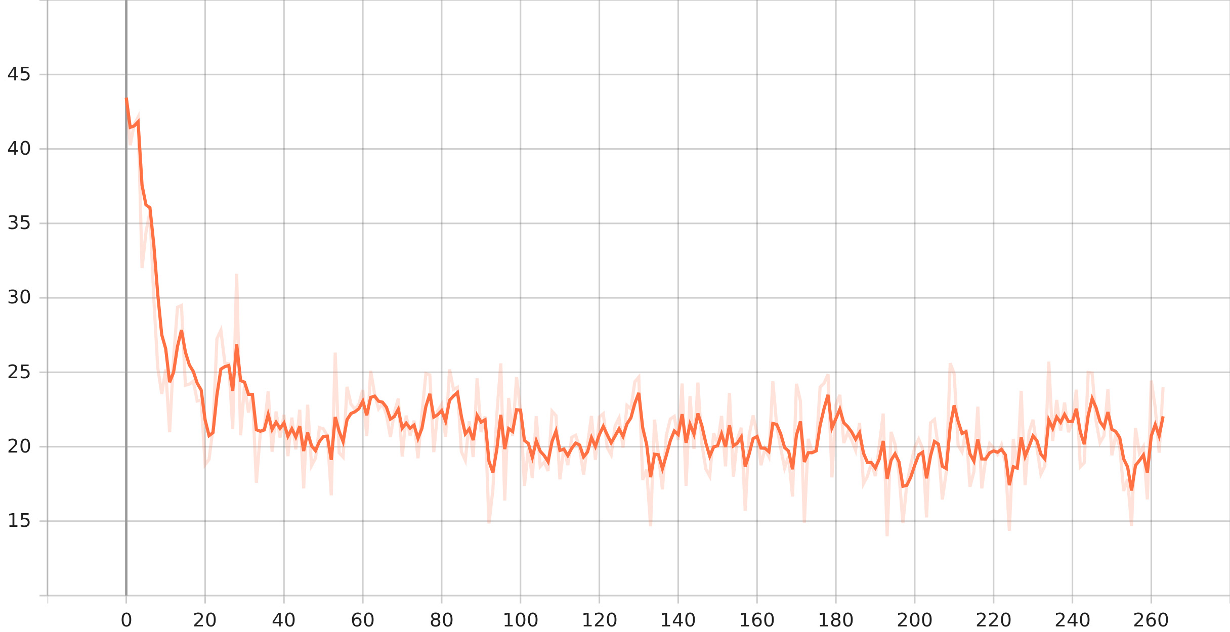
We ran the model against the target pawpularity score which provided us an RMSE score of \(19.187\)
Below is the plot of RMSE loss in terms of epoch. As we can see the from the training loss plot, we
are able to reduce the RMSE from \(40\) to \(20\) using the above model.
[Fig 7] Training loss change with epochs
Final validation RMSE turns out to be \(19.18\) which means there is not much of performance boost from
the deep neural model.
Attempt 2: Tuned Imagenet
Our next attempt was to train deep vision architectures that are pre-trained on ImageNet dataset and
finetune the network to the Petfinder
pawpularity dataset. We used Pytorch Image models (timm) to obtain the pre-trained ImageNet models
and used them as the
backbone feature extractor in the finetuning.
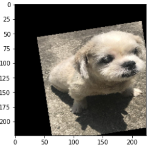
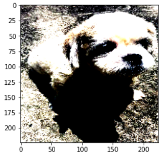
We obtained the pet image dataset after the duplicate removal and performed several
transforms/augmentations to improve
the model robustness and enhance the dataset size. Some examples of different transforms we
experimented with are given below:
Original Image:
Horizontal/ Vertical flip
Random Affine transformation
Mild Color jittering
Normalization with ImageNet Statistics:
We observed that normalization is negatively affecting the training objective as this would
generate visually off-putting images for humans but with high popularity scores and essentially
confusing and hampering the training of the network
Training details:
Since training the deep computer vision architectures is expensive both in terms of time and
compute power, we limited ourselves to the below experimentation and hyperparameter tuning to
obtain the best model.
Model Architectures:
We experimented with the below models and replaced the final classification
head with the fully connected regressor head which outputs the final pawpularity
value.
EfficientNet-B0
EfficientNet-B4
Resnet18
Swin Transformer
Hyper parameter tuning:
Below are the major hyper parameters we experimented / tuned to obtain the optimal
architecture:
Training / Validation batch sizes:
We experimented with the batch sizes of \(32,64,128\) for both the training and
validation datasets. Changing the batch size did not affect the validation loss
significantly for our experiments.
Learning Rate:
We experimented with initial learning rates ranging from \(1\times 10^{-5}\) to
\(1\times 10^{-3}\) and then use learning rate schedulers to control
the learning rate during the training.
LR Schedulers:
We tried the below lr scheduler settings available in the pytorch framework
We observed that starting with a higher learning like 1e-3 along with the stepLR
scheduler with a gamma of 0.9 achieved the better validation loss results among
all the settingsedulers to control the learning rate during the training.
Optimizer:
We experimented with optimizers such as 1) SGD with momentum, adaptive
optimizers like 2) Adam and 3) AdamW(weight decay). In our observations, Adam
consistently resulted in better training loss across all the architectures.
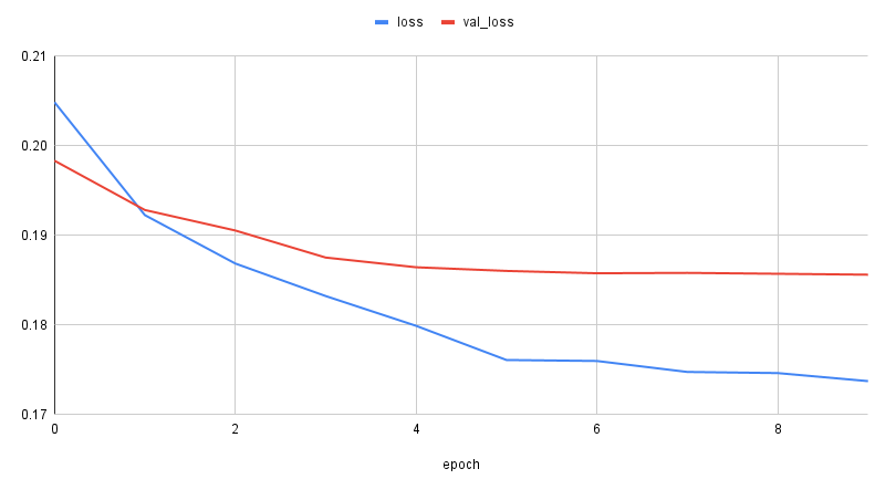
Results:
Best model configuration: We achieved the best validation RMSE of 18.67 using the below architecture and hyper parameter
settings.
[Fig 8] Train and Validation RMSE
Attempt 3: Pretrain on Oxford-IIIT
After ImageNet results, we felt that the model needs to be pre-trained on some pet dataset so that
it can learn to understand the heuristics for assigning pawpularity score in our target dataset. We
used the Oxford-IIIT [9] dataset to pre-tune a EfficientNet_b4 from scratch on breed detection task for
both cats and dogs and then fine-tune it on our pawpularity dataset. Our assumption here was that
the breed of the dog plays a major factor in deciding the pawpularity score and while learning to
breed the pre-trained model will also learn to understand minute features in pets. Note that this
assumption is quite different from our ImageNet approach where we gave lighting conditions and
background image a higher priority in assigning the score.
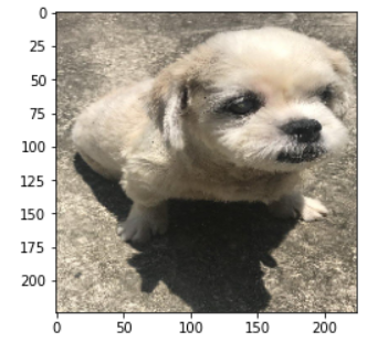
As before, we obtained the pet image dataset after the duplicate removal and performed several
transforms/augmentations to improve the model robustness and enhance the dataset size. Some examples
of the Oxford-IIIT dataset images are:
Oxford-IIIT details:
The dataset contains 37 categories of dogs and cat breeds with roughly 200 images for each
class. The images have large variations in scale, pose and lighting. The ground truth labels
used for pre-training were the breed of animal.
ImageNet Architectures:
We used the EfficientNet_b4 model for pre-training task by attaching a linear head
for breed classification. After
pre-training we repeat our configuration for ImageNet model by removing the last
layer and attaching a fully connected
regressor head which outputs the final pawpularity score.
Hyper parameter tuning:
Below are the major hyper parameters we experimented / tuned to obtain the optimal
architecture:
Training / Validation batch sizes:
We experimented with the batch sizes of \(16, 32, 64\) for both the training and
validation datasets. As before, changing the
batch size did not affect the validation loss significantly for our experiments
but it did affect the rate of training.
We used a batch size of 64 for finally reporting our performance.
Learning Rate:
We experimented with initial learning rates of \(1\times 10^{-2}\) and then used
Exponential
Learning rate decay scheduler (default parameter settings) to control the
learning rate during the training.
Optimizer:
We trained our model with Adam optimizer in its default parameter settings of
tensorflow.
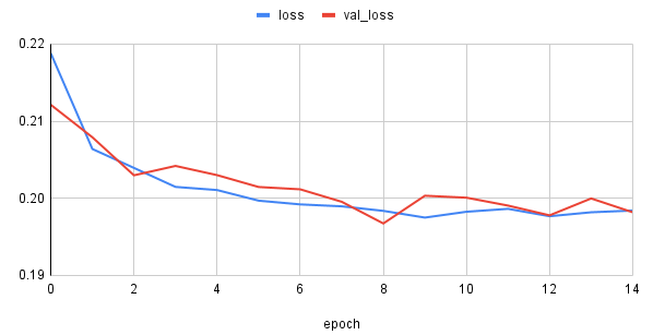
Results:
Best model configuration: We achieved the best validation RMSE of 19.67 using the
below architecture and hyper parameter
settings.
ImageNet
Architecture
EfficientNet_b4
Training/Val
data size ratio
4:1
Epochs
10
Training/Val
batch size
64
Learning
Rate
1e-2
Optimizer
Adam
LR
Scheduler
Exponential
decay
[Fig 9] Change of loss with epoch
Deep learning models results comparison
Architectures
Weights
Duplicate images
Optimizer
Batch Size
Train-test split
Epochs
Learning rate
Multi step
RMSE
EfficienNet-B0
Encoder Frozen
(ImageNet)
Untouched
SGD
24
90 to 10
10
1.00E-03
epochs: [5, 8], gamma:
0.1
19.2
Fully trainable
(ImageNet)
Untouched
SGD
24
90 to 10
10
1.00E-03
epochs: [5, 8], gamma:
0.1
18.7
Fully trainable
(ImageNet)
Duplicates set to max
score of 2
SGD
24
90 to 10
10
1.00E-03
epochs: [5, 8], gamma:
0.1
18.72
Fully trainable
(ImageNet)
Duplicates set to max
score of 2
SGD
24
90 to 10
10
1.00E-03
epochs: [5, 8], gamma:
0.1
18.68
EfficienNet-B4
Fully
trainable(ImageNet)
Untouched
Adam
64
4 to 1
10
1.00E-03
step epoch: 1, gamma:
0.9
18.67
Fully trainable
(pretrained from Oxford IIT breed dataset)
Duplicates
removed
Adam
64
4 to 1
10
1.00E-02
Exponential
delay
19.67
Resnet18
Encoder Frozen
(ImageNet)
Untouched
Adam
64
4 to 1
10
1.00E-03
step epoch: 1, gamma:
0.9
19.17
Swin Transformer
Fully trainable
(ImageNet)
Untouched
Adam
64
4 to 1
10
1.00E-03
step epoch: 1, gamma:
0.9
19.8
Results and discussions
After trying different data modalities (meta-data and images), architectures, pre-training datasets
and hyperparameters
we compile our result in the following table. Note that lower the RMSE, better is the model in
predicting the
pawpularity score.
Method
RMSE
Linear Regression
20.4944
Linear
Regression with PCA
20.4777
LightGBM
20.4667
Pretrained ImageNet with frozen weights
19.187
ImageNet with finetuned weights
18.67
Oxford IIIT
19.67
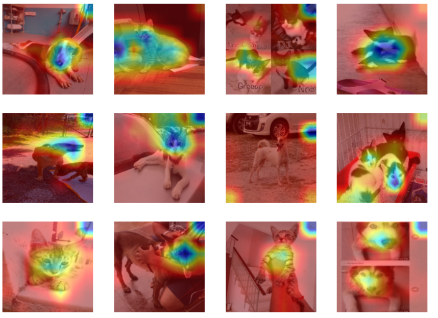
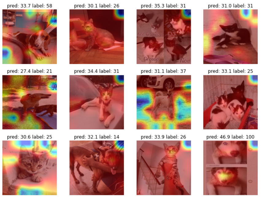
GradCAM++ Visualizations:
To further analyze the cause of our performance we made, we tried to visualize the gradients learned
by the best performing network to
understand where the network is focussing on to produce the popularity score. We used GradCAM++(
Generalized Gradient-based Visual Explanations for Deep Convolutional Networks ) [8] module
supported by the Pytorch framework to achieve this.
[Fig 10] GradCAM++ visualizations obtained by the directly pretrained ImageNet
models
[Fig 11] GradCAM++ visualizations after fine tuning the network for
PetPawpularity prediction
Observations:
From the above visualizations, we can clearly see that initially, the focus of the
pre-trained network was on the pets
(i.e. face/body of the pet) which will help in the classification task. After the
finetuning, it started focussing more
on the background clutter which intuitively makes sense that background information is
being more helpful in determining
the pawpularity score of the image
Conclusion
The data exploration stage gave us a clear insight that meta-data isn’t discriminating against
different pawpularity
scores and hence, is a very noisy data. We shifted our focus to using images directly for predicting
the score and
tested various deep learning methods with various initializations and hyperparameters. By comparing
the performance
obtained between ImageNet initialization and Oxford-IIIT dataset initialization, we can infer that
the pawpularity score
depends heavily on the extrinsic features like the background of the image, the objects on the pet,
lighting conditions
etc. instead of the breed of the pet itself. Based on this result, we can conclude with reasonable
certainty that the
chances of a pet getting adopted increases if the photograph is taken in a good lighting condition,
perhaps with some
pet-friendly objects irrespective of the breed of the pet.
All team members contributed equally towards the completion of this project. We appreciate the help by the teaching staff team throughtout the course. Cheers!